The objective of this node is to explain Analysis of Algorithms and Asymptotic Notations i.e. Big-O, Omega-Ω, and Theta-Θ. These topics are the most basic foundation for Data Structures and Algorithms.
Analysis of Algorithms
The idea of analysis of algorithms is to compare algorithms mainly in terms of running time and space consumed.
For example,
To go from city 'M' to city 'N', there can be many ways to carry-out this task: by flight, by bus, by train and also by bicycle. Depending on the accessibility and convenience, we choose the one that suits us. Similarly, in computer science we have various algorithms available for solving a same problem, for example we can solve sorting problem by many algorithms like selection-sort, bubble-sort, merge-sort and many more but we will choose the one with lesser complexity. (Best algorithm for sorting is quick-sort with complexity O(nlog(n)) )
This concludes that Analysis of Algorithm should be used in determining which method is more efficient and also which method is good in terms of time and space consumed.
Prior to learning Asymptotic Notations, Let's see what is rate of growth of an algorithm.
Rate of growth is nothing but the rate at which the run time complexity of the algorithm increases as a function of the input.
Let's suppose we have to purchase a laptop and a mouse. If someone asks you what are you purchasing, then in general you will say buying a laptop and ignore buying the mouse part. This is because, cost of laptop is too big compared to cost of mouse. So, we can say
Total Cost = cost_of_laptop + cost_of_mouseTotal Cost ≈ cost_of_laptop (approximately)For the above mentioned example, we can represent the cost of laptop and cost of mouse as a function and for a given function, we can ignore the lower order terms (that are relatively insignificant for large value of input size, n). Let us consider another example in terms of algebra, let n4, n2, 100n and 5 are individual costs of some function, here we can approximate this function to n4 i.e. the highest rate of growth.
n4 + n2 + 100n + 5 ≈ n4
Here's the list of most common rate of growths.
| Time Complexity | Name | Example |
| 1 | Constant | accessing an array element |
| log(n) | Logarithmic | finding an element in a sorted array |
| n | Linear | finding an element in a unsorted array |
| nlog(n) | Linear Logarithmic | sorting n items with divide-and-conquer (Merge Sort) |
| n2 | Quadratic | shortest path between two nodes in a graph |
| n3 | Cubic | matrix multiplication |
| 2n | Exponential | tower of hanoi problem |
Before going to Asymptotic Notations, We also need to know about Types Of Analysis.
Types of Analysis
If we have to analyse an algorithm, we need to know on what inputs the algorithm takes less time, and on what inputs the algorithm is taking more time. That means we can represent algorithms with multiple expressions: one for the case where it takes less time and other for the case where it takes more time.
In general, when the algorithm takes less time it is called as the best case and when the algorithm takes more time than it is called as the worst case.
To analyse an algorithm we need some kind of syntax and that forms the base for asymptotic analysis / notation.
There are three types of analysis:
- Worst Case
- defines the input for which algorithm takes longest time to execute.
- algorithm runs slower.
- algorithm which executes maximum number of steps on input data of size n.
Best Case
- defines the input for which algorithm takes lowest time to execute.
- algorithm runs fastest.
- algorithm which executes least number of steps on input data of size n.
Average Case
- provides a prediction about the running time of the algorithm.
- assumes that the input is random.
- algorithm which performs average number of steps on input data of size n.
Lower Bound <= Average Time <= Upper BoundAsymptotic Notations
Asymptotic Notations is having an expressions for the best, average and worst cases, for all the three cases we need to identify the upper and lower bounds. To represent these upper and lower bounds we need some kind of syntax and that is the following discussion. Let us assume that for a given algorithm, it can be represented in the form of function f(n).
Big - O Notation :
This notation gives the tight upper bound of the given algorithm / function f(n). It is represented as
f(n) = O(g(n)).
It means, for larger values of n, the upper bound of function f(n) is a function g(n).
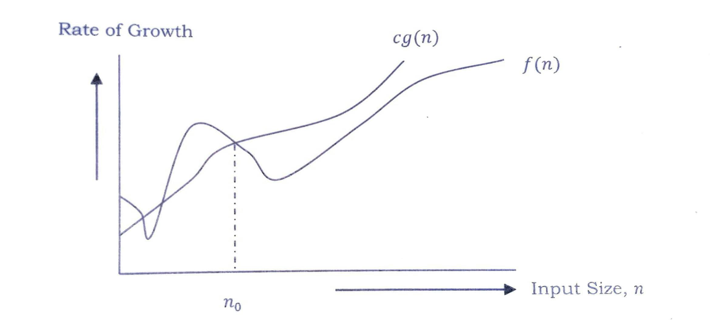
Here upper bound means, value of f(n) cannot exceed g(n) after a particular value of n. (represented as n0 in the graphical approach).
Let's see this with a graphical approach.

After n = n0, value of g(n) is always greater than or equal to the given algorithm's rate of growth f(n).
Also, for example, if f(n) = n4 + 100n + 50 is the given algorithm, then n4 is g(n). That means, g(n) = n4 gives the maximum rate of growth for f(n) at larger values of n.
O-Notation can be also be defined as O(g(n)) = { f(n) : there exists positive constant c and n0 such that 0 ≤ f(n) ≤ cg(n) for all n ≥ n0 }.
Our objective is to get smallest rate of growth g(n) which is greater than or equal to f(n)'s rate of growth.
Generally we discard lower values of n. That means the rate of growth at lower values of n is not important. In the graph, n0 is the point from which we need to consider the rate of growths for a given algorithm. Below n0 the rate of growths could be different.
Some Big - O Examples:
f(n) = n2 + 1
n2 + 1 ≤ 2n2, for all n ≥ 1
Therefore, n2 + 1 = O(n2), with c = 2 and n0 = 1
f(n) = 2n3 - 2n2
2n3 - 2n2 ≤ 2n3, for all n ≥ 1
Therefore, 2n3 - 2n2 = O(2n3), with c = 2 and n0 = 1
There is one more thing related to values of n0 and c, that is, there is no isolated set of values for n0 and c in finding the asymptotic bounds. Let us see an example, 100n + 5 = O(n). For this function, there can be multiple values for n0 and c, giving us an asymptotic solution / bound.
Solution 1 : 100n + 5 ≤ 100n + n = 101n, for all n ≥ 5, n0 = 5 and c = 101.
Solution 2 : 100n + 5 ≤ 100n + 5n = 105n, for all n ≥ 1, n0 = 1 and c = 105.
Both possibilities are correct.
Note : Most of the time we are interested in knowing the Big - O Notation i.e. Tight Upper Bound of an algorithm because it allows us to estimate weather an algorithm is feasible for our application or not, by telling us that this algorithm will not take more than such-and-such amount of memory or time when run on an input of size n.
Omega - Ω Notation :
This notation gives the tight lower bound of the given algorithm / function f(n). We can represent it as
f(n) = Ω(g(n))
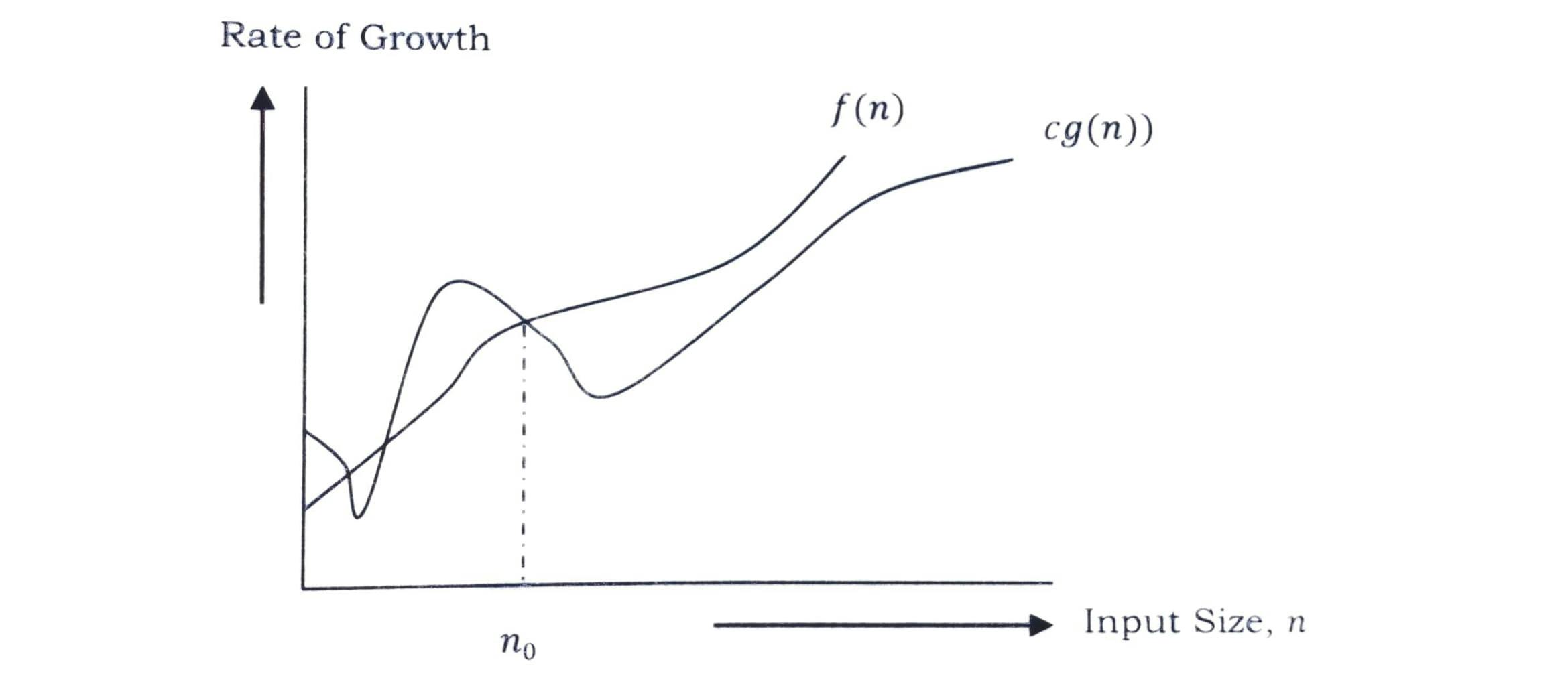
It means, for larger values of n, g(n) is the lower bound of function f(n).
Here lower bound means, rate of growth of f(n) is always greater than or equal to the rate of growth of function g(n) after a particular value of n i.e. n0.
Let's see this with a graphical approach.

After n = n0, value of g(n) is always smaller than or equal to the given algorithm's rate of growth f(n).
Ω Notation can also be defined as Ω(g(n)) = { f(n) : there exists positive constants n0 and c such that 0 ≤ cg(n) ≤ f(n) for all n ≥ n0 }.
Here, our objective is to get largest rate of growth g(n) which is less than or equal to f(n)'s rate of growth. g(n) is asymptotic lower bound for the given algorithm's rate of growth f(n).
Some Ω Examples :
f(n) = 5n2
∃ (there exists) c, n0, such that: 0 ≤ cn ≤ 5n2 => c = 1 and n0 = 1
Therefore, 5n2 = Ω(n2)
2n = Ω(n), n3 = Ω(n3), logn = Ω(logn)
Note : Lower bounds are of great use as well. Lower bounds can give information about whether we can improve our algorithm or is it feasible. We can also know that our algorithm is optimal, if our lower bound is equal to the upper bound.
Theta - Θ Notation :
This notation gives a range of upper bound and lower bound and determines whether the upper bound and lower bound of the given algorithm are same. The average running time of an algorithm is always between the lower bound (Omega - Ω) and upper bound (Big - O) of the function. If the upper bound and lower bound of a function gives the same result (rate of growth) then Theta - Θ will also have the same rate of growth.
For example, assume f(n) = 10n + n, then its tight upper bound is O(n) and the lower bound is Ω(n). In this case, rate of growths in the best case and worst case are same. As a result, the average case will also be the same. If for a given algorithm, the rate of growths O and Ω are not same then the rate of growth for Θ may not be same. In this case, we have to consider all possible time complexities and take average of those. (for example, quick sort average case gives Θ(nlogn) complexity)
Let us also see this in a graphical approach.

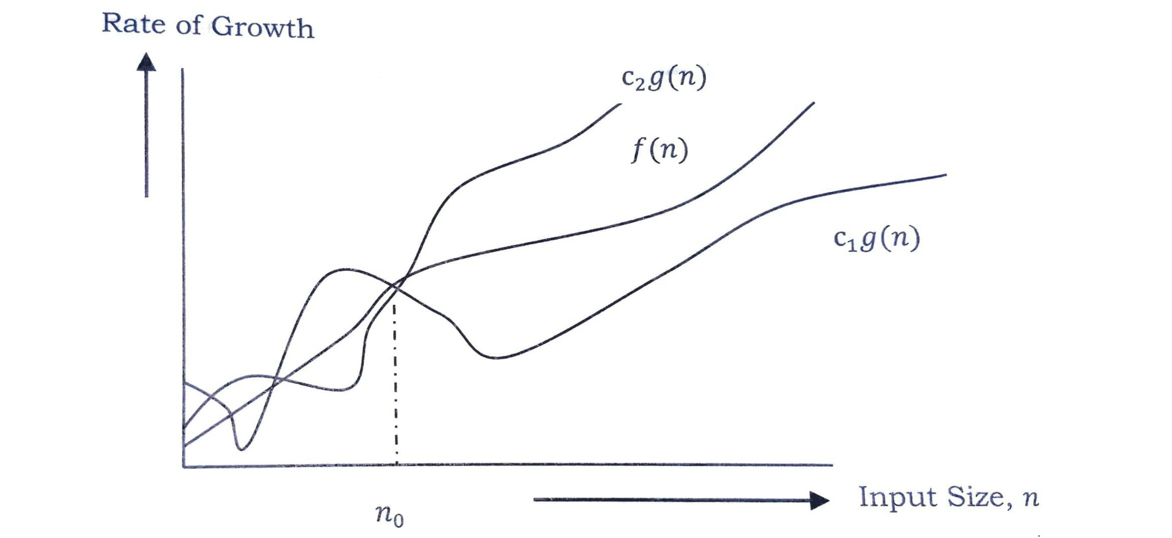
After n = n0, the value of f(n) is always between c2g(n) and c1g(n).
Θ Notation can also be defined as Θ(g(n)) = { f(n) : there exists positive constants c1, c2, and n0 such that* 0 ≤ c1g(n) ≤ f(n) ≤ c2g(n) , for all n ≥ n0 }. g(n) is an asymptotic tight bound for f(n).
Θ(g(n)) is a set of functions with same order of growth as g(n).
Some Θ Examples:
Prove n ≠ Θ(n2)
c1n2 ≤ n ≤ c2n2, only holds for n ≤ 1 / c1
Therefore, n ≠ Θ(n2)
Prove 6n3 ≠ Θ(n2) c1n2 ≤ 6n3 ≤ c2n2, only holds for n ≤ c2 / 6
Therefore, 6n3 ≠ Θ(n2)
Why is it called Asymptotic Notations?
For all the three notations, O, Ω, Θ, in every case for a given function f(n) we are trying to find other function g(n) which approximates f(n) at large values of n. That means, g(n) is also a curve which approximates f(n) at large values of n.
In mathematics, we call such curves as asymptotic curves. In other terms, g(n) is the asymptotic curve for f(n). For this reason, we call algorithm analysis as asymptotic analysis and notations as asymptotic notations
Properties of Notations:
- Transitivity : f(n) = Θ(g(n)) and g(n) = Θ(h(n)), then f(n) = Θ(h(n)). Valid for O and Ω as well.
- Reflexivity : f(n) = Θ(f(n)). Valid for O and Ω as well.
- Symmetry : f(n) = Θ(g(n)) if and only if g(n) = Θ(f(n)).
- Transpose symmetry : f(n) = O(g(n)) if and only if g(n) = Ω(f(n)).
Bonus :
Master Theorem for Divide and Conquer
All divide and conquer algorithms works by dividing the problem into sub-problems, each of which is part of the original problem and then we perform some additional work to compute the final answer. As an example, merge sort algorithm operates on two sub problems, each of which is half the size of the original problem and then performs O(n) additional work for merging the sub-problems.
This gives the running time of the equation :
T(n) = 2T(n / 2) + O(n)
Master theorem can be used to determine the running time of divide and conquer algorithms. For a given algorithm, first we try to find the recurrence relation of the problem. If the recurrence relation is of the below form then we can directly give the answer without fully solving it.
If the recurrence relation is of the form, T(n) = aT(n / b) + Θ(nklogpn), where a ≥ 1, b > 1, k ≥ 0 and p is a real number, then:
If a > bk, then T(n) = Θ(nlogab)
If a = bk
a. If p > -1, then T(n) = Θ(nlogablogp+1n).
b. If p = -1, then T(n) = Θ(nlogabloglogn).
c. If p < -1, then T(n) = Θ(nlogab)If a < bk
a. If p ≥ 0, then T(n) = Θ(nklogpn)
b. If p < 0, then T(n) = O(nk)
